Perfecting Imperfections: A Journey in Warping Objects into Circles

Disclaimer

This example details the basics of the method; the code is not optimized for production and serves solely as an example. Several parts can be vectorized and effectively utilize NumPy arrays. A production ready version can be found here.

Problem Statement

Identifying nearly circular objects within images and refining them into perfectly round shapes while preserving their natural appearance is our goal. This is particularly relevant in iris art photography for example, where the iris, though not naturally perfectly circular, can be enhanced by maintaining its integrity while achieving a more symmetrical form. Two minutes of video are captured using the smartphone, while simultaneously recording the heart rate using a TomTom ECG chest strap and a Wahoo Element device. The goal is to compare the average heart rate observed during this two-minute test.

Challenge

Our task is twofold: accurately detecting almost circular objects within images and transforming them into perfect circles without distorting their intricate patterns.

Detection

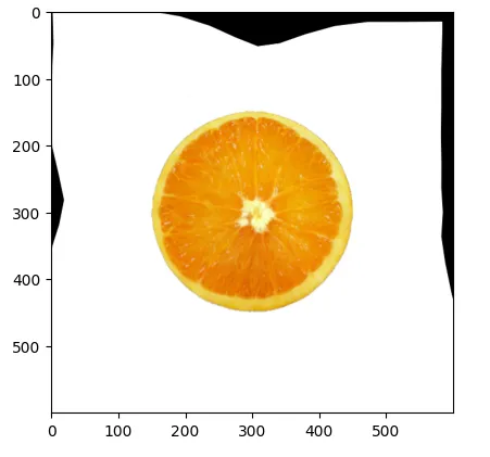
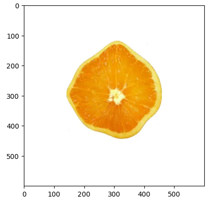
The initial step is to generate a binary mask of the object, in our scenario, a deformed orange. We can accomplish this with simple thresholding. However, for more complex objects, employing advanced segmentation models like YOLO (You Only Look Once) may be necessary.

original = cv2.cvtColor(cv2.imread("orange.png"), cv2.COLOR_BGR2RGB) 
plt.imshow(original)
    

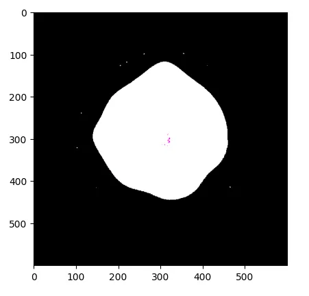
_, image = cv2.threshold(original, 254, 255, cv2.THRESH_BINARY_INV)
plt.imshow(image)
    

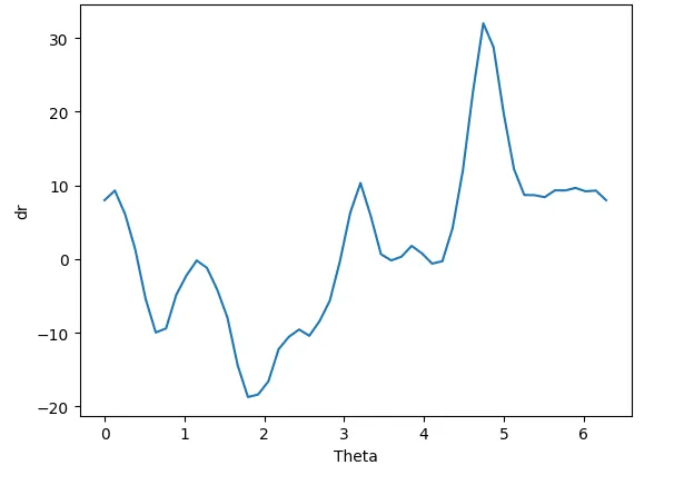
Following that, we utilize OpenCV contour detection to identify the object boundaries. The critical step of the algorithm entails discretizing our space using polar coordinates with parameters N_RADIUS and N_THETA and leveraging this grid to warp the image.

Initially, we calculate the distance between the circle radius and the shape of the object for each discrete radius. This distance yields a positive value if the object border lies outside the circle, and negative otherwise. For simplicity, we employ the Shapely library to compute this distance.

# Find contours
contours, _ = cv2.findContours(image[:, :, 0], cv2.RETR_TREE, cv2.CHAIN_APPROX_SIMPLE)
contours = sorted(contours, key=cv2.contourArea)
contours = np.squeeze(contours[-1])
contours[-1] = contours[0] # close polygon
contours = shapely.LineString(contours)

# Parameters for discretizing space into polar coordinates
N_THETA = 50
N_RADIUS = 15
theta = np.linspace(0, 2*np.pi, N_THETA)
r = np.linspace(0, 600, N_RADIUS)

# Define circle parameters
CIRCLE_RADIUS = 150
CIRCLE_CENTER = 300

# Compute distance between circle radius and object shape for each discrete radius
delta_r = []
for i in theta:
    intersection = shapely.intersection(shapely.LineString([[CIRCLE_CENTER,CIRCLE_CENTER], [CIRCLE_CENTER+500*np.cos(i), CIRCLE_CENTER+500*np.sin(i)]]), contours)
    dr = shapely.distance(intersection, shapely.Point([CIRCLE_CENTER, CIRCLE_CENTER])) - shapely.distance(shapely.Point([CIRCLE_CENTER+CIRCLE_RADIUS*np.cos(i), CIRCLE_CENTER+CIRCLE_RADIUS*np.sin(i)]), shapely.Point([CIRCLE_CENTER, CIRCLE_CENTER]))
    delta_r.append(dr)

plt.plot(theta, delta_r)
plt.xlabel("Theta")
plt.ylabel("dr")
    

Transformation

The concluding step involves determining the method by which we will deform the space so that the object shape ends up as a circle while preserving its internal geometry. For each discrete radius, our objective is to map the coordinates of the object shape on this radius to the circle’s radius, with the center of the object aligning with the center of the radius. To accomplish this, we can opt for an affine function as outlined below.

def f(r, dr):
    return (CIRCLE_RADIUS/(CIRCLE_RADIUS+dr))*r
    

We will utilize the computed grid with parameters N_RADIUS and N_THETA, along with the corresponding deformed grid obtained using the transformation described earlier. Each point of the original grid will be mapped to its corresponding point in the transformed grid.

# Original grid
X = []
Y = []
for j in theta:
    for i in r:
        X.append(i*np.cos(j) + CIRCLE_CENTER)
        Y.append(i*np.sin(j) + CIRCLE_CENTER)

# Transformed grid
X_ = []
Y_ = []
for l, i in enumerate(theta):
  for k, j in enumerate(r):
    r_ = f(j, delta_r[l])
    X_.append(r_*np.cos(i) + CIRCLE_CENTER)
    Y_.append(r_*np.sin(i) + CIRCLE_CENTER)

plt.scatter(X, Y, color="blue", label="Original grid")
plt.scatter(X_, Y_, color="red", label="Transformed grid")
plt.xlim(0,600)
plt.ylim(0,600)
plt.legend()
    

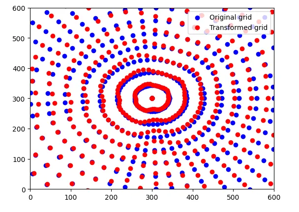
Image Warping

Subsequently, we employ a piecewise affine transformation to execute the image warping process, resulting in the final image.

src = np.dstack([X, Y])[0]
dst = np.dstack([X_, Y_])[0]
tform = PiecewiseAffineTransform()
tform.estimate(dst, src)
out = warp(original, tform)
plt.imshow(out)